Motivation:

Before diving into the actual material, it's important to find the core drive behind learning linear algebra. Lots of us (including myself) took linear algebra courses in the college, but we never really understood how it's useful, and why we needed to learn it in the first place.
Most likely, our remnant knowledge of linear algebra was reduced to numerical operations between 2-3 vectors, e.g. how to compute determinant using diagnal rules, how to compute dot product of 2 vectors...... This is pure sadness.
After watching Terrence Tao's master class, I had some sort of epiphany, mathematics should be a method to guide you to transform your way of thinking, finding a narrative or a story for your problem. Especially there are several great examples from Terrance's class:

• Kepler measured the wine volume in a wine barrel -> finding the local maximum;
• measuring the salt content of sea -> sampling population (why the size of population is not as important);
• Transforming the game of finding 15 (magic square), to playing tic-tac-toe; $\begin{bmatrix} 2 & 7 & 6 \\ 9 & 5 & 1 \\ 4 & 3 & 8 \\ \end{bmatrix}$
• Counterfeit coin problem (12 coins, 1 scale, 3 times limitation) -> Linear algebra -> Compress Sensing

Resources

• Gilbert Strang, god of Linear Algebra. This course reignited my desire to learn math.
  
  
• This essence series is pure magic, beyond words to describe how helpful it is.
  
  
• Zico's Review is the most concise written version. Fundamentals;
  
  Matrix Calculus:
  Jacobian: $f: \mathbb{R}^n \rightarrow \mathbb{R}^m$, $D_x f(x) \in \mathbb{R}^{m \times n}$
  $(D_x f(x))_{ij} = \frac{\partial f_i(x)}{\partial x_j}$
  Gradient:$f: \mathbb{R}^n \rightarrow \mathbb{R}$, $\nabla_x f(x) = \begin{bmatrix} \frac{\partial f(x)}{\partial x_1} \\ \frac{\partial f(x)}{\partial x_2} \\ \vdots \\ \frac{\partial f(x)}{\partial x_n} \end{bmatrix}= (D_x f(x))^T$
  Hessian:$f: \mathbb{R}^n \rightarrow \mathbb{R}$, $\nabla^2_x f(x) = \mathbb{R}^{n \times m} = D_x (\nabla_x f(x)) = \begin{bmatrix} \frac{\partial^2 f(x)}{\partial x_1\partial x_1} &\frac{\partial^2 f(x)}{\partial x_1\partial x_2} &\cdots &\frac{\partial^2 f(x)}{\partial x_1\partial x_n} \\ \frac{\partial^2 f(x)}{\partial x_2\partial x_1} & & & \\ \vdots &\ddots & &\vdots \\ \frac{\partial^2 f(x)}{\partial x_n\partial x_1} & & & \frac{\partial^2 f(x)}{\partial x_n^2} \end{bmatrix} $
  Symmetric by construction, $f(x) = X^T Ax, x \in \mathbb{R}^n, A \in \mathbb{R}^{n \times m}$, $\nabla_x f(x) = (A + A^T) x$, $\nabla_x^2 f(x) = A + A^T $
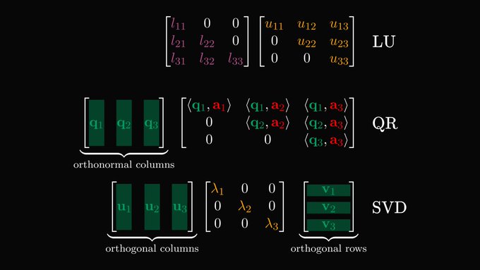LU, QR, SVD (Image Credit)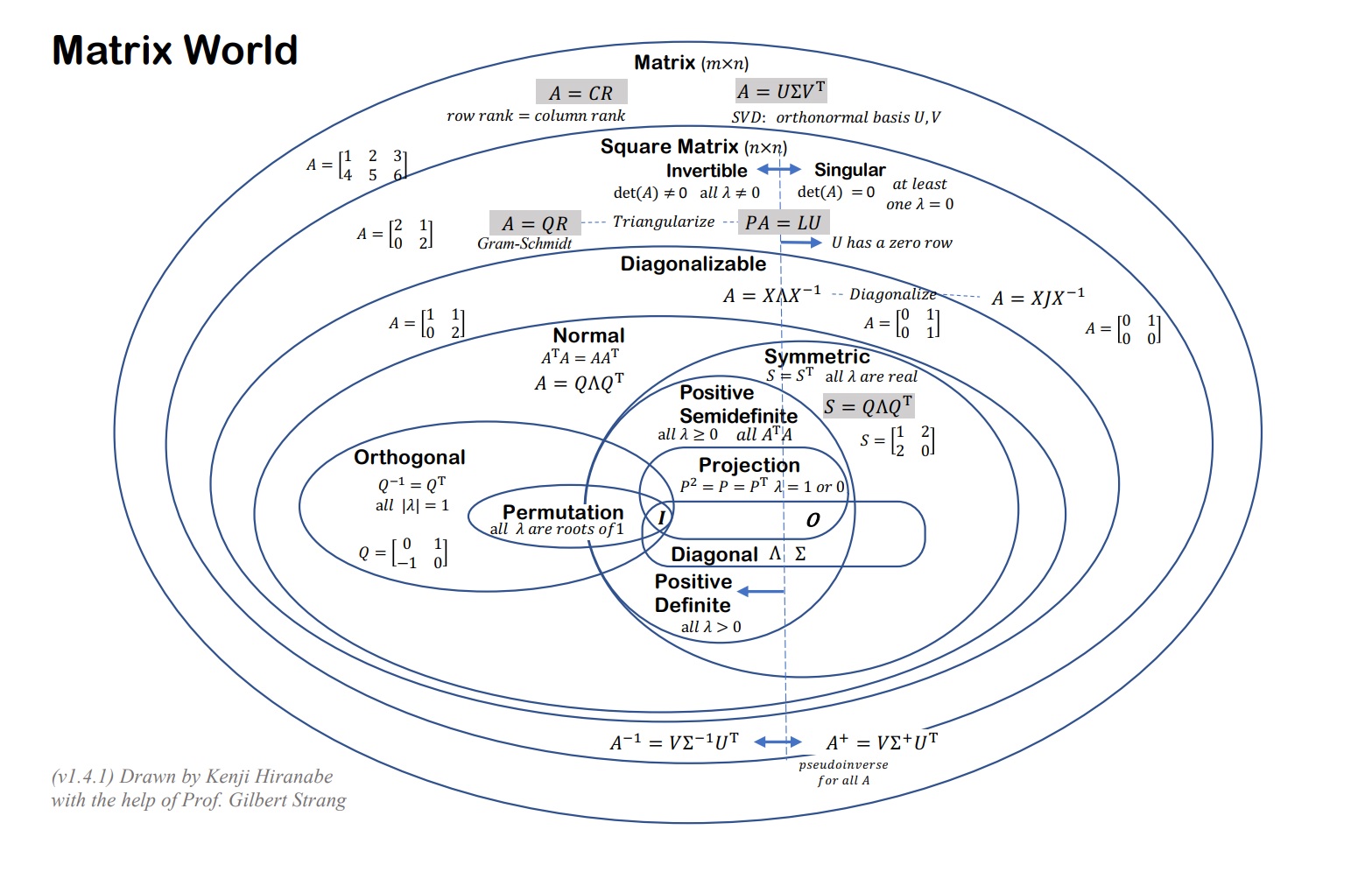

Interesting Facts:

1. Projection: $$P^2 = P,\\ P^T = P,\\ P = A(A^TA)^{-1}A^T, \\ A\hat{X}= A(A^TA)^{-1}A^Tb$$ Why did we need $proj.$ to begin with? Since $Ax=b$ might not have a solution, so we instead solve proj of b onto the column space $Ax = p$
   If b in column space, $Pb = b$
   If b $\perp$ column space, $Pb = 0$ (in the null space of $A^T$)
\( \newcommand{\rotvert}{\rotatebox[origin=c]{90}{$\vert$}} \newcommand{\rowsvdots}{\vdots} \newcommand{\brows}[1]{% \begin{bmatrix} \begin{array}{@{\protect\rotvert\;}c@{\;\protect\rotvert}} #1 \end{array} \end{bmatrix} } \)
2. QR decomposition (Gram Schmidt):
   Orthonomal vectors: $q_i^T \cdot q_j = \begin{cases} 1 & \text{if i $\neq$ j }\\ 0 & \text{if i = j} \end{cases}$
   $ Q^T Q = \brows{q_1^T \\ q_2^T \\ \rowsvdots \\ q_n^T} \begin{bmatrix} \vert & \vert \\ \vec{q_1} & \vec{q_n} \\ \vert & \vert \end{bmatrix} = \begin{bmatrix} 1 & & & \\ & 1 & & \\ & & \ddots & \\ & & & 1 \end{bmatrix}=I $ $$A = QR,\\ Q^{-1} = Q^T,\\ QRx = b,\\ Rx = Q^Tb$$
3. Determinant: $Det(I) = 1$,
   Det is linear to each row! Det(
   $Det(2A) = 2^nDet(A)$,$Det(AB) = Det(A)Det(B)$, $Det(A) = Det(A^T)$,$Det(LU) = Det(L^T)Det(U^T)$, $Det(A^{-1}) = \frac{1}{Det(A)}$, $Det(A^{-1})Det(A) = 1$ Exchange rows reverse sign of Det
4. Eigenvalues and eigenvectors:
   Intuition: multiply by $A$ doesn't change the direction, instead just scales it. $A \in \mathbb{R}^{n\times n}, x \in \mathbb{C}^n, \lambda \in \mathbb{C}$
   at most you could have $n$ independent eigen values and $n$ eigen vectors
   $Ax = \lambda x$
   $AX = X\Lambda \Leftrightarrow A = X\Lambda X^{-1}$ (if $X$ invertible), where $\Lambda = \begin{bmatrix} \lambda_{1} & & & \\ & \lambda_{2} & & \\ & & \ddots & \\ & & & \lambda_{n} \end{bmatrix}$
   $A^2 = X\Lambda X^{-1}X\Lambda X^{-1} = X\Lambda^{2}X^{-1}$
   What can we say about $A^k$ when $k \rightarrow \infty$?
   As long as there's one eigen value $> 1$, gets to $\infty$. VS. Every eigen value $<1$, $A^k \rightarrow 0$

Fourier

FFT in action, the best video about FFT out there:

Derivation of FFT in action

STFT, DFT, FFT everything... A wonderful lecture.

Using FFT to process audio with librosa, making use of stft, and power_to_db. Librosa

Fun edge case when doing fft on a masked signal. Step Fourier

Translating Math to code

A Tensor Puzzle that contains almost all fancy operation one can do in PyTorch about linear algebra.

Solving Image overlap question using Linear algebra, Leetcode 835.

Hardware Acceleration of Linear Algebra, how to break down the $O(n^3)$ matrix multiplication operation to loading cost, register cost, and speed them up.