Basic Theory Notebook and pointers
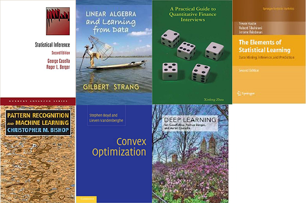
Being a researcher to work on A.I (apologize for using the buzz word), apart from coding skills, one really gotta have to be equipped with a solid background in math and stats. Nobody, maybe except for senior PhDs in math or stats major can claim that they know everything, but at least we need those basic intuitions to understand how an algorithm works, or where the theoretical guarantee comes from. Here are the 7 books I have read.
- Cassella Book is a must, where you know your bounds, distribution, and where RV comes from.
- Strang's Linear Algebra doesn't need much of my own explanation
- This "Green book" is really a good pointer to all the basics.
- Bishop book is the bible of ML.
- Boyd book is probably the most practical book out there about optimization. Rockfella one is too hard for me.
- Statistical Learning book is also very famously fundamental.
- Goodfellow book is new, but not necessarily the best written one.
- Expected Value, Variance and Covariance
- Common Families of Distributions
- Useful Inequalities
- Convergence of sequence
- Regression
Expected Value, Variance and Covariance
If you claim you know stats, and you flounder at any of the above questions... great embarrassment.
Covariance and Correlation derivationIf $X_1, \ldots, X_n$ are independent then: $ {\sf Var}\left(\sum_{i=1}^n a_i X_i\right) = \sum_i a_i^2 {\sf Var}\left(X_i\right). $
The sample mean is $$ \widehat{\mu}_n = \frac{1}{n}\sum_i X_i $$ Why sample variance has a divider of (n-1)? $$ \widehat{\sigma}^2_n= \frac{1}{n-1} \sum_i (X_i- \widehat{\mu}_n)^2. $$ The sampling distribution of $\widehat{\mu}_n$ is $$ G_n(t) = \mathbb{P}(\widehat{\mu}_n \leq t). $$ LeetCode528 talks about inverse CDF sampling. $X_i = F^{-1}(U_i).$ $U_1,\cdots,U_n$ independently with distribution U[0,1]
Sample to draw
Reparameterization trick done right
- Choose a coordinate to update, uniformly at random, i.e. with probability $\frac{1}{n}$ we select co-ordinate $j$.
- Update its value by sampling from the conditional distribution keeping all other coordinates fixed, i.e. we sample a new value for $x_j$ : $x_j \sim \pi(x_j |(x_1, . . . , x_{j−1}, x_{j+1}, . . . , x_n))$.
Common Families of Distributions
Useful Inequalities
-
Inequality Cheetsheet
- Markov Inequality The most elementary tail bound is Markov's inequality, which asserts that for a positive random variable $X \geq 0$, (only for non-negative!) \begin{align*} \mathbb{P}(X \geq t) \leq \frac{\mathbb{E}[X]}{t}. \end{align*}
- Chebyshev Inequality Chebyshev's inequality states that for a random variable $X$, with ${\sf Var}(X) = \sigma^2$: \begin{align*} \mathbb{P}( |X - \mathbb{E}[X]| \geq k \sigma) \leq \frac{1}{k^2}~~~~\forall k \geq 0. \end{align*} Proof: Chebyshev's inequality is an immediate consequence of Markov's inequality. \begin{align*} \mathbb{P}( |X - \mathbb{E}[X]| \geq k \sigma) &= \mathbb{P}( |X - \mathbb{E}[X]|^2 \geq k^2 \sigma^2) &\leq \frac{\mathbb{E}(|X - \mathbb{E}[X]|^2)}{k^2 \sigma^2} = \frac{1}{k^2}. \end{align*} Good enough for constant-probability statements. Things usually are around a few standard deviations. Only requires pairwise independence.
- Define, $\mu = \mathbb{E}[X]$. For any $t > 0$, we have that, \begin{align*} \mathbb{P}((X - \mu) > u) = \mathbb{P}( \exp(t(X - \mu)) > \exp(t u) ) \leq \frac{ \mathbb{E}[\exp(t(X - \mu))]}{\exp(t u)}. \end{align*} Now $t$ is a parameter we can choose to get a tight upper bound, i.e. we can write this bound as: \begin{align*} \mathbb{P}((X - \mu) > u) \leq \inf_{0 \leq t \leq b} \exp (-t(u + \mu)) \mathbb{E}[\exp(tX)]. \end{align*} This bound is known as Chernoff's bound.
- Formally, a random variable $X$ with mean $\mu$ is sub-Gaussian(tails decay faster than Gaussian) if there exists a positive number $\sigma$ such that, \begin{align*} \mathbb{E}[\exp(t(X - \mu))] \leq \exp (\sigma^2 t^2/2), \end{align*} for all $t \in \mathbb{R}$. Gaussian random variables with variance $\sigma^2$ satisfy the above condition with equality, so a $\sigma$-sub-Gaussian random variable basically just has an mgf that is dominated by a Gaussian with variance $\sigma$.
- Jensen's inequality: Jensen's inequality states that for a convex function $g: \mathbb{R} \mapsto \mathbb{R}$ we have that, \begin{align*} \mathbb{E}[g(X)] \geq g(\mathbb{E}[X]). \end{align*} If $g$ is concave then the reverse inequality holds.
- This in turn yields Hoeffding's bound. Suppose that, $X_1,\ldots, X_n$ are independent identically distribution bounded random variables, with $a \leq X_i \leq b$ for all $i$ then, \begin{align*} \mathbb{P}\left( \left| \frac{1}{n} \sum_{i=1}^n X_i - \mu \right| \geq t \right) \leq 2 \exp \left( - \frac{nt^2}{(b-a)^2} \right). \end{align*} This is a two-sided exponential tail inequality for the averages of bounded random variables.
- Bernstein's inequality suppose we had $X_1,\ldots,X_n$ which were i.i.d from a distribution with mean zero, bounded support $[a,b]$, with variance $\mathbb{E}[(X-\mu)^2] = \sigma^2$. Then, \begin{align*} \mathbb{P}(| \widehat{\mu} - \mu| \geq t) \leq 2 \exp\left( - \frac{nt^2}{2(\sigma^2 + (b-a) t)} \right). \end{align*} Roughly this inequality says with probability at least $1 - \delta$, \begin{align*} |\widehat{\mu} - \mu| \leq 4 \sigma \sqrt{ \frac{\ln (2/\delta)}{n}} + \frac{ 4(b-a) \ln(2/\delta)}{n}. \end{align*} Intuition: both subgaussian (near the mean) and subexponential (far tails) parts: "Poisson-like" bounds.
- The union bound. This is also known as Boole's inequality. It says that if we have events $A_1,\ldots,A_n$ then \begin{align*} \mathbb{P}\left( \bigcup_{i=1}^n A_i\right) \leq \sum_{i=1}^n \mathbb{P}(A_i). \end{align*}
- Levy's inequality/Tsirelson's inequality: Concentration of Lipschitz functions of Gaussian random variables: \begin{align*} |f(X_1,\ldots,X_n) - f(Y_1,\ldots,Y_n)| \leq L \sqrt{\sum_{i=1}^n (X_i - Y_i)^2}, \end{align*} for all $X_1,\ldots,X_n,Y_1,\ldots,Y_n \in \mathbb{R}$. For such functions we have that if $X_1,\ldots,X_n \sim N(0,1)$ then, \begin{align*} \mathbb{P}(|f(X_1,\ldots,X_n) - \mathbb{E}[f(X_1,\ldots,X_n)] | \geq t) \leq 2 \exp \left( - \frac{t^2}{2L^2} \right). \end{align*}
- A $U$-statistic is defined by a kernel, which is just a function of two random variables, i.e. $g: \mathbb{R}^2 \mapsto \mathbb{R}$. The U-statistic is then given as: \begin{align*} U(X_1,\ldots,X_n) := \frac{1}{ {n \choose 2} } \sum_{j < k} g(X_j, X_k). \end{align*} e.g. Variance: $g(X_j, X_k) = \frac{1}{2}(X_j-X_k)^2$ Mean Absolute Deviation $g(X_j, X_k) = |X_j-X_k|$.
- Mcdiarmid's Inequality Formally, we have i.i.d. RVs $X_1,\ldots,X_n$, where each $X_i \in \mathbb{R}$. We have a function $f: \mathbb{R}^n \mapsto \mathbb{R},$ that satisfies the property that: \begin{align*} |f(x_1,\ldots,x_n) - f(x_1,\ldots,x_{k-1}, x'_k, x_{k+1},\ldots,x_n)| \leq L_k, \end{align*} for every $x,x' \in \mathbb{R}^n$, i.e. the function changes by at most $L_k$ if its $k$-th coordinate is changed. This is known as the bounded difference condition. If the random variables $X_1,\ldots, X_n$ are i.i.d then for all $t \geq 0$ \begin{align*} \mathbb{P}(|f(X_1,\ldots,X_n) - \mathbb{E}[f(X_1,\ldots,X_n)] | \geq t) \leq 2 \exp \left( - \frac{2t^2}{\sum_{k=1}^n L_k^2} \right). \end{align*} For bounded $U$-statistics, i.e. if $g(X_i, X_j) \leq b$, we can apply Azuma's inequality to obtain a concentration bound. Note that since each random variable $X_i$ participates in $(n-1)$ terms we have that, \begin{align*} |U(X_1,\ldots,X_n) - U(X_1,\ldots,X_i',\ldots, X_n)| \leq \frac{1}{{n \choose 2}} (n-1)(2b) = \frac{4b}{n}. \end{align*} So that Azuma's inequality tells us that, \begin{align*} \mathbb{P}(|U(X_1,\ldots,X_n) - \mathbb{E}[U(X_1,\ldots,X_n)] | \geq t) \leq 2 \exp (-nt^2/(8b^2)). \end{align*} Pinsker's Inequality is cancelled
Concetration Inequality short video
Concentration Inequality Slides
Johnson–Lindenstrauss (JL) lemma states that you can efficiently transform many very big things into many much smaller things, and it's OK.
Deviation from the mean
Convergence of Sequence
- Almost sure convergence \begin{align*} \lim_{n \rightarrow \infty} X_n = X. \end{align*} The correct analogue turns out to be to require: \begin{align*} \mathbb{P}\left(\lim_{n \rightarrow \infty} X_n = X\right) = 1. \end{align*}
- Convergence in probability: A sequence of random variables $X_1,\ldots,X_n$ converges in probability to a random variable $X$ if for every $\epsilon > 0$ we have that, \begin{align*} \lim_{n \rightarrow \infty} \mathbb{P}( |X_n - X| \geq \epsilon) = 0. \end{align*} Example: Weak Law of Large Numbers Suppose that $Y_1,\ldots,Y_n$ are i.i.d. with $\mathbb{E}[Y_i] = \mu$ and $\text{Var}(Y_i) = \sigma^2 < \infty$. Define, for $i \in \{1,\ldots,n\}$, \begin{align*} X_i = \frac{1}{i} \sum_{j = 1}^i Y_j. \end{align*} The WLLN says that the sequence $X_1,X_2,\ldots$ converges in probability to $\mu$. {\bf Proof: } The proof is simply an application of Chebyshev's inequality. We note that by Chebyshev's inequality: \begin{align*} \mathbb{P}(|X_n - \mathbb{E}[X]| \geq \epsilon) \leq \frac{\sigma^2}{n \epsilon^2}. \end{align*} This in turn implies that, \begin{align*} \lim_{n \rightarrow \infty} \mathbb{P}(|X_n - \mathbb{E}[X]| \geq \epsilon) = 0, \end{align*} as desired. Usually we will construct an estimator $\widehat{\theta}_n$ for some quantity $\theta^*$. We will then say that the estimator is consistent if the sequence of RVs $\widehat{\theta}_n$ converges in probability to $\theta^*$.
- Convergence in Quadratic Mean: \begin{align*} \mathbb{E}(X_n - X)^2 \rightarrow 0, \end{align*} as $n \rightarrow \infty$.>
- Convergence in Distribution: We say that a sequence converges to $X$ in distribution if: \begin{align*} \lim_{n \rightarrow \infty} F_{X_n}(t) = F_X(t), \end{align*} for all points $t$ where the CDF $F_X$ is continuous.
5 ways to do linear Regression
- Least Square method and it's derivation and an intuitive example.
- Matrix Formulation for Multiple Linear Regression, but need to understand Matrix Derivation
- Projection Matrix
- Weighted Least Square:
We would like to fit a linear regression model to the dataset $ \mathcal{D} = \left\{\left(\mathbf{x}^{(1)},y^{(1)}\right), \left(\mathbf{x}^{(2)},y^{(2)}\right),\cdots, \left(\mathbf{x}^{(N)},y^{(N)}\right)\right\} $ with $\mathbf{x}^{(i)} \in \mathbb{R}^M$ by minimizing the ordinary least square (OLS) objective function: $ J(\mathbf{w}) = \frac{1}{2}\sum_{i=1}^N\left(y^{(i)} - \sum_{j=1}^M w_j x_j^{(i)}\right)^2 $ Specifically, we solve for each linear regression coefficient $w_k, 1\leq k\leq M$, by deriving an expression for $w_k$ from the critical point $\frac{\partial J(\mathbf{w})}{\partial w_k} = 0$. expression for each $w_k$: $w_k = \frac{\sum_{i=1}^N x_k^{(i)}\left(y^{(i)}-\sum_{j=1,j\neq k}^M w_j x_j^{(i)}\right)}{\sum_{i=1}^N \left(x_k^{(i)}\right)^2}$
$\hat{\beta}_{WLS} = \underset{\beta}{argmin}{\sum\limits_{i=1}^n{\epsilon_i^2}} = (X^T WX)^{−1}X^T WY$
Comments
Want to leave a comment? Visit this post's issue page on GitHub (you'll need a GitHub account).